Forecasting Danish Pharmaceutical Exports
A univariate 24-month forecast of Denmark's monthly pharmaceutical exports through the GLP-1 boom, comparing SARIMA and ETS under a diagnostics-first selection gate. The whole paper is built on one principle: a forecast is only as good as its prediction intervals, so statistical validity is gated before accuracy. CBS Predictive Analytics final project, 2026.
Overview
Denmark is the EU's 8th-largest pharmaceutical exporter (≈ €13.7 bn, 2024), and pharma is roughly 30% of Danish goods exports. The series is statistically interesting precisely because it is hard: monthly exports nearly doubled between 2022 and 2026, driven by GLP-1 (weight-loss) demand and Novo Nordisk in particular — a possible regime shift on top of strong seasonality and non-constant variance.
This project builds and validates univariate time-series forecasts on DST Statbank data (SITC 54, Jan 2007 – Mar 2026, 231 monthly observations), comparing the ARIMA/SARIMA family against ETS exponential smoothing, with seasonal naïve as the MASE baseline. Univariate is a deliberate scope choice — it tests how far the series' own history takes you, and it is the honest baseline because external predictors (GLP-1 sales, capacity) aren't known in advance.
Research question
Can a univariate time-series model, estimated using the fpp3 framework, produce a diagnostically valid and accurate 24-month forecast of Danish pharmaceutical exports?
Data
DST Statbank, SITC 54 (medicinal & pharmaceutical products), nominal DKK, Jan 2007 – Mar 2026 (231 obs). The series rises from 2.6–4.0 Bn DKK/month (2007) to 15–19 Bn DKK/month (2025–26). 🔗 Dataset: pharma_exports.csv (231 monthly rows) — extracted from the Statistics Denmark Statbank (SITC 54).
| Period | Mean | Min | Max | Std. dev. |
|---|---|---|---|---|
| Full sample (2007–2026) | 8.33 | 2.60 | 18.87 | 4.03 |
| Pre-2022 (2007–2021) | 6.69 | 2.60 | 10.89 | 1.82 |
| Post-2022 (2022–2026) | 14.10 | 8.91 | 18.87 | 2.41 |
Descriptive statistics (Bn DKK). The post-2022 jump is a broad level shift, present in every calendar month.
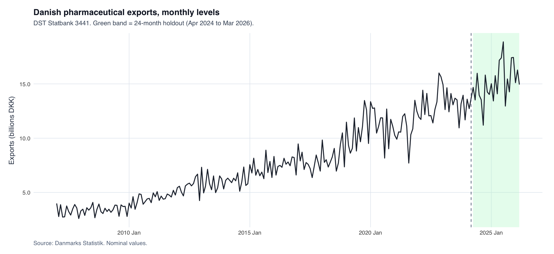
Monthly export levels, 2007–2026. The green band is the 24-month holdout (Apr 2024 – Mar 2026); the steep post-2022 climb is the GLP-1 boom the model is asked to forecast.
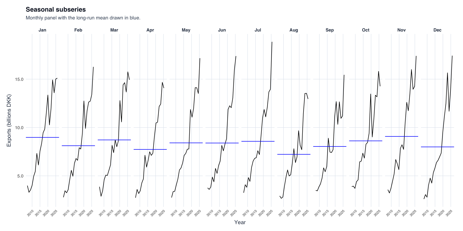
Seasonal subseries plot. The post-2022 acceleration appears in every calendar month — evidence it's a level shift, not a change in seasonal structure (which justifies no seasonal differencing).
Transformation & stationarity
- Box-Cox (Guerrero): λ = −0.0177 ≈ 0 → natural log throughout. Seasonal swings grow with the level; logging stabilises variance and makes additive seasonality on the log scale ≈ multiplicative on the original scale.
- Differencing:
ndiffs = 1,nsdiffs = 0→ one regular difference, no seasonal differencing (seasonal amplitude is stable, so seasonal AR/MA at lag 12 captures it without throwing away data).
| Test | Series | p-value | Interpretation |
|---|---|---|---|
| KPSS | log(exports) | 0.01 | Non-stationary → d = 1 |
| ADF | log(exports) | 0.31 | Unit root not rejected |
| ADF | diff(log) | 0.01 | Stationary after differencing |
KPSS and ADF have opposite nulls, so using both is a robustness cross-check. Structural breaks: QLR/sup-F on diff(log) finds no break (p = 1.00); indicator saturation (gets::isat) flags only Dec 2012/Jan 2013 at 1%; Bai-Perron (BIC) selects 0 breakpoints. First-differencing already removes the level shift, so the acceleration is smooth and sustained, not a discrete break.
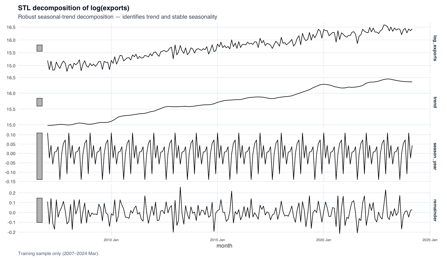
STL decomposition of log(exports): a smooth rising trend and a stable-amplitude seasonal component — the two facts that drive the d = 1, D = 0 specification.
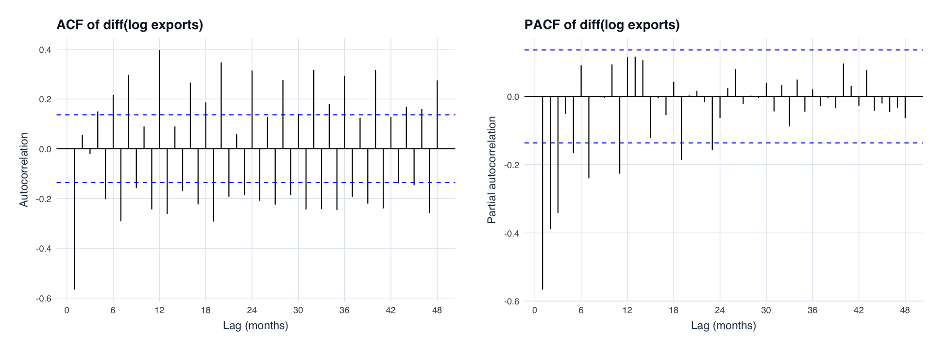
ACF/PACF of the differenced log series. The lag-1 (and small lag-2) ACF spikes point to MA(1)/MA(2); the lag-12 spike to a seasonal MA; PACF decay at seasonal lags to a seasonal AR — this is how the (0,1,2)(1,0,1)[12] orders were identified by hand.
Train–test split
| Set | Period | N |
|---|---|---|
| Training | 2007M01 – 2024M03 | 207 |
| Holdout (test) | 2024M04 – 2026M03 | 24 |
All orders and hyperparameters were fixed on the training set before the holdout was touched. The April 2024 cutoff deliberately puts the entire GLP-1 boom in the test set — a hard test, and the project's real safeguard against an unmodelled regime change.
Methodology — the two-stage gate
- Stage 1 — diagnostic validity (a hard gate): a model must return a Ljung-Box p > 0.05 at lags 12 and 24. Autocorrelated residuals mean unreliable 80%/95% prediction intervals, so such models are excluded regardless of accuracy.
- Stage 2 — out-of-sample accuracy: among models that pass, the ARIMA winner and ETS winner go head-to-head on holdout RMSE/MAE/MAPE/MASE plus rolling-origin cross-validation over 19 origins.
No cross-class AIC ranking is used: ARIMA and ETS likelihoods are computed on different bases and are not comparable. Information criteria are used only within each class.
Results
ARIMA candidates
| Model | AICc | LB p (lag24) | RMSE | MAPE |
|---|---|---|---|---|
| ARIMA(0,1,1)(1,0,1)[12] | −415 | 0.093 | 1.62 | 8.65% |
| ARIMA(0,1,2)(1,0,1)[12] | −417 | 0.363 | 1.73 | 8.85% |
| ARIMA(1,1,1)(1,0,1)[12] | −416 | 0.271 | 1.69 | 8.76% |
| auto.ARIMA | −399 | 0.155 | 2.02 | 9.58% |
All four candidates pass Ljung-Box at 5%; (0,1,2)(1,0,1)[12] has the lowest AICc and the widest LB margin → carried forward. Hand identification beat the automatic search, which was worst on every metric.
ETS candidates
| Model | AICc | LB p (lag24) | RMSE | MAPE |
|---|---|---|---|---|
| ETS(A,A,A) | 106 | 0.124 | 1.69 | 8.92% |
| ETS(A,Ad,A) / Auto ETS | 96 | 0.037 | 2.36 | 11.71% |
Only ETS(A,A,A) passes Ljung-Box. Auto ETS picks the damped trend (better AICc) but fails diagnostics and degrades the post-2022 forecast.
Head-to-head & rolling cross-validation
| Model | LB p (lag24) | Holdout RMSE | CV RMSE | MASE |
|---|---|---|---|---|
| SARIMA(0,1,2)(1,0,1)[12] | 0.363 | 1.73 | 1.66 | 1.28 |
| ETS(A,A,A) | 0.124 | 1.69 | 1.70 | 1.26 |
| Seasonal naïve (baseline) | — | — | 1.92 | 1.00 |
On the single holdout ETS is marginally ahead, but SARIMA wins rolling CV (19 origins, stretch window) on all three averaged metrics and has the wider Ljung-Box safety margin (0.363 vs 0.124) → more reliable intervals. A ~2% point-accuracy gap on one split isn't decisive; CV over 19 origins is. We don't overclaim — ETS(A,A,A) is a close, valid reference, and their near-identical performance validates the benchmark design.
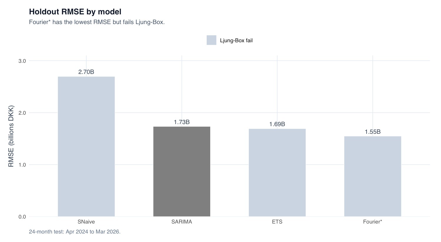
Holdout RMSE by model. The lowest bar (ARIMA + Fourier, 1.55 Bn) is the one we reject — it fails Ljung-Box, so the gate disqualifies it despite winning on raw error. This chart is the visual argument for diagnostics-first.
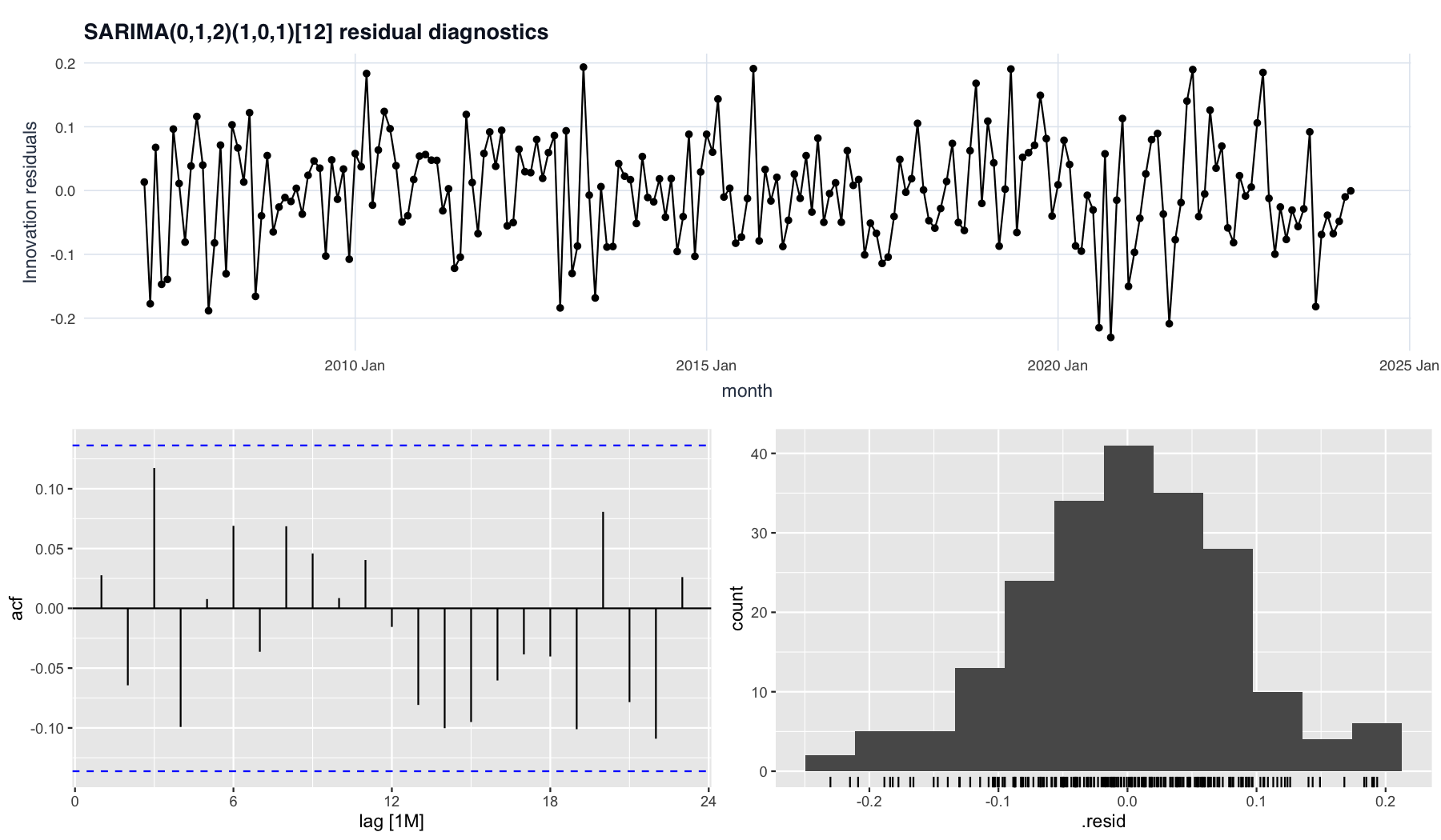
Residual diagnostics for the chosen SARIMA: ACF bars sit inside the 95% bands (clean white noise) and the residual histogram is roughly symmetric — the basis for trustworthy prediction intervals.
Excluded by the gate: ARIMA + Fourier(K=2) had the lowest holdout RMSE (1.55 Bn) but failed Ljung-Box (p≈0). Three SARIMAX variants (GLP-1/COVID step dummies) all failed at lag 24 and added no accuracy — the drift had already absorbed the smooth trend, so a one-off step dummy is the wrong shape and adds noise.
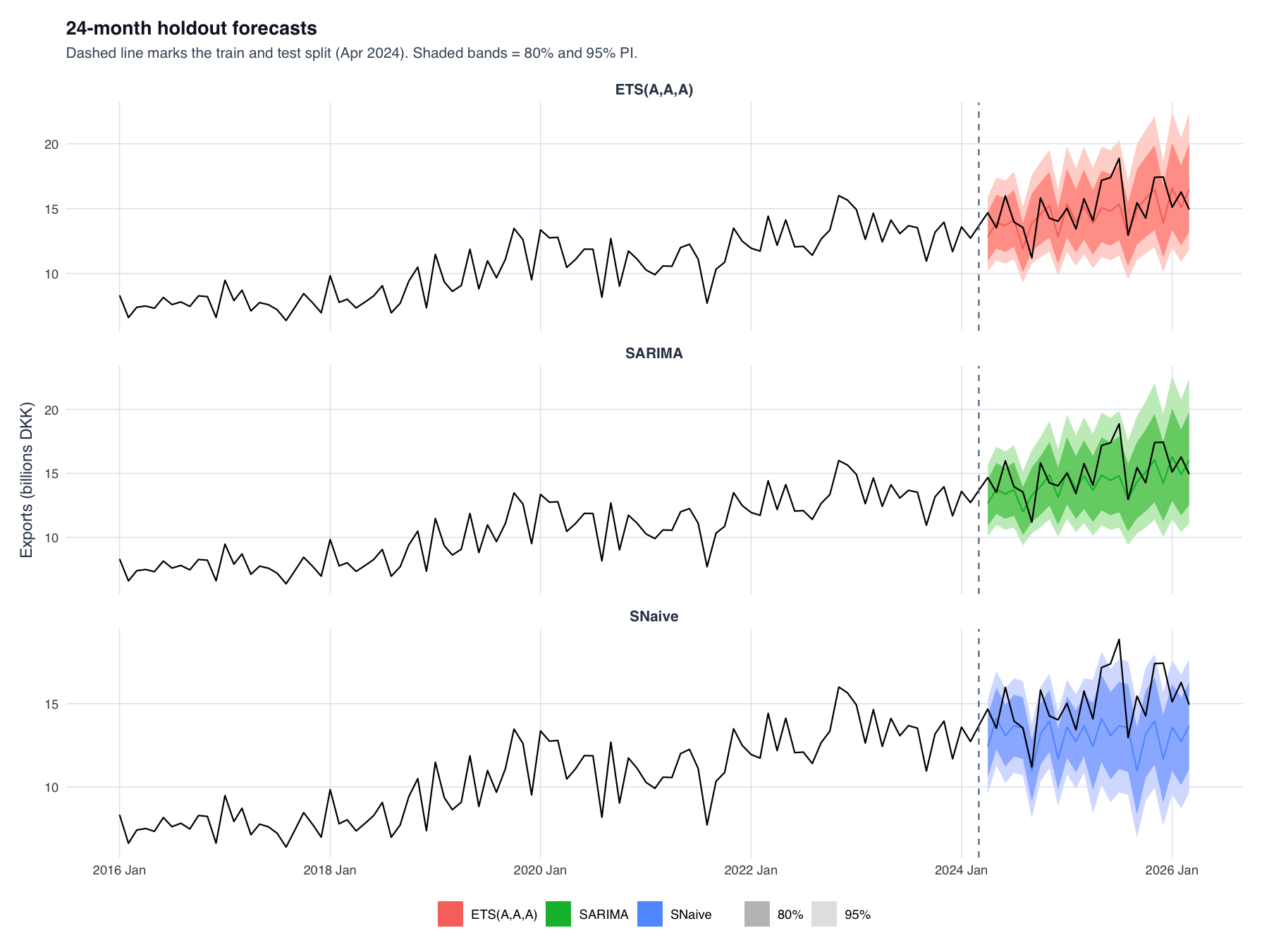
The 24-month holdout forecasts. Both SARIMA and ETS track the trend and under-predict the steepest part of the boom; seasonal naïve flatlines on last year's values, showing why it gives no usable forward signal.
The chosen model & forecast
ARIMA(0,1,2)(1,0,1)[12] with drift (ma1 = −0.926, ma2 = +0.166, sar1 = 0.974, sma1 = −0.845). The drift is kept despite t ≈ 1 because out-of-sample behaviour, not a single t-stat, is the test — dropping it makes the long-horizon forecast flatten and under-shoot the real trend. Forecast: ≈ 17 Bn DKK/month by early 2026; 80% PI ≈ 15.0–19.5, 95% PI ≈ 13.5–21.0 Bn DKK. Honest caveat: MASE = 1.28 > 1, so on this boom holdout the model is marginally worse than a naïve month-to-month guess on point accuracy — the value is in the trend and reliable intervals, and SARIMA still beats naïve in CV (1.66 vs 1.92).
Key takeaways
- Diagnostics-first beats chasing the lowest error: the lowest-RMSE model (Fourier) was excluded for failing Ljung-Box — its intervals would be untrustworthy.
- Step dummies added no value: the drift already absorbed the smooth, sustained level shift, so a one-off dummy added noise, not signal.
- Biggest threat is concentration: the "macro" series is largely one firm (Novo Nordisk); a capacity or competitor shock is invisible to a univariate model, so we lean on intervals over the point forecast.
Reasoning behind the modelling choices
Each decision follows the same logic: a characteristic of the data justifies a choice, and rules out an alternative.
| Characteristic of the series | What it justifies | Rejected alternative (and why) |
|---|---|---|
| Seasonal swings grow with the level | Log / Box-Cox (λ ≈ 0) | Raw scale → growing variance breaks ARIMA/additive-ETS assumptions |
| Unit root on level, stationary after 1 difference | d = 1 | d = 0 → spurious trend; d = 2 → over-differenced |
| Seasonal pattern stable in amplitude | D = 0, seasonal AR/MA at lag 12 | Seasonal difference → removes a pattern that isn't changing |
| Clear, smooth, sustained uptrend | Drift term (kept despite t ≈ 1) | Step dummy → wrong shape for a gradual shift |
| Acceleration is gradual, not a jump | No break dummy (QLR/Bai-Perron agree) | SARIMAX dummies → fail Ljung-Box, no OOS gain |
| Forecast used through its intervals | Diagnostics-first gate | Lowest-RMSE Fourier → invalid intervals, disqualified |
If a structural break existed but went unmodelled? A level shift (our case) is handled by first-differencing. A slope break would make the fixed drift over/under-shoot increasingly with horizon — you'd need a time-varying trend. A variance break would mis-size the intervals. Putting the whole boom in the holdout already stress-tests this: the model still produced valid residuals and reasonable intervals out of sample.
Limitations & future work
- Limitations: Novo Nordisk dominance → single-firm proxy; nominal DKK (no real/price adjustment); ETS LB p = 0.124 passes but isn't large → monitor; boom-period results may not generalise to calmer conditions.
- Future work: firm/product-level data to break the single-firm proxy; a time-varying external regressor (e.g. a production/capacity index) via dynamic regression instead of a fixed step dummy; Bayesian structural time series; forecasting growth rates rather than levels.
Dataset & downloads
Dataset (CSV) Final paper (PDF) Repository on GitHub
Related Projects
- Bachelor Thesis — quantitative statistical modelling in R
- Banana Ripeness Classification — deep learning, CBS Data Science 2026
- Echo Chamber Linguistics — NLP text classification, CBS Data Science 2026